Extended Game of Life
- 22 Nov 2020
- Manuel Capel
- Tags: miscellanous
Invented by Conway in 1970, the game of life is a quite fascinating application of cellular automata with deep implications in computer science and mathematics. Let’s just see here how to make a pretty flexible multi-valued and multi-dimensional implementation of them leveraging numpy.
1
2
3
4
5
6
7
8
import numpy as np
from matplotlib import pyplot as plt
from matplotlib import colors
import imageio
from IPython.display import display, Image

cmap = colors.ListedColormap(['blue', 'white', 'red'])
N = 15
We begin with defining a NxN grid with random integer values in (0, 1, 2) on its squares:
1
2
arr = np.random.randint(3, size=N * N, dtype=np.int8)\
    .reshape(N, N)
Then for each value we define:
- the surrounding for cells in the grid having this value
- the rules to apply for these cells
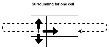
If we take for example [(1, 0), (-1, 0), (0, 1), (0, -1)] as surrounding/neigborhood for the cells in state 0 at the current step, it means that for each of those cells, at position say p, we will sum the values of the cells located at p + (1, 0), p + (-1, 0), p + (0, 1) and p + (0, -1). If the a surrounding cell lands over the edge, it continues on the other side.

The transitions correspond to the mapping of this sum to (0, 1, 2). For example, transitions_0 = [((0, 1), 1), ((2, 3), 1), ((4, np.inf), 0)] means that if 0 <= sum <=1 then the concerned cell will turn to value 1, if 2<= sum <=3 then the concerned cell will turn to value 1 also, if sum >=4 it will turn to 0.
1
2
3
4
5
6
7
8
9
10
11
12
13
14
15
16
17
18
19
20
21
22
23
24
# Tuple ind surroundings must have at most
# as many elements as dimensions in `arr`
surrounding_0 = [(1, 0), (-1, 0),
                    (0, 1), (0, -1)]
surrounding_1 = [(1, 1), (-1, -1),
                    (-1, 1), (1, -1)]
surrounding_2 = [(1, 1), (-1, -1),
                    (-1, 1), (1, -1)]

transitions_0 = [((0, 1), 1),
                 ((2, 3), 1),
                 ((4, np.inf), 0)]
transitions_1 = [((0, 2), 0),
                 ((3, 3), 1),
                 ((4, np.inf), 1)]
transitions_2 = [((0, 2), 2),
                 ((3, 4), 1),
                 ((4, np.inf), 0)]

rules = {
 0: (surrounding_0, transitions_0),
 1: (surrounding_1, transitions_1),
 2: (surrounding_2, transitions_2)
}
Note: Here and in the following, we use completely arbitrary sets of surroundings (a.k.a. neighborhoods) and transitions for the cells. surrounding_k (resp. transitions_k) denotes the set of surroundings/neighbors (resp. transitions) applicable to cells have value/state k at the current step.
This way you can create any set of rules on any set of states instead of the three rules on 2 states of the original Conway’s game of life, also rules implying very distant cells, as you wish.
Now we define a few functions to compute each step of the evolution of the grid:
1
2
3
4
5
6
7
8
9
10
11
12
13
14
15
16
17
18
19
20
21
22
23
24
25
26
27
28
29
30
31
32
33
34
35
36
37
38
39
40
41
42
43
44
45
46
47
48
49
50
51
52
53
54
55
56
57
58
59
60
61
62
63
64
65
# Tuple ind surroundings must have
# at most as many elements as dimensions in `arr`
surrounding_0 = [(1, 0), (-1, 0),
                 (0, 1), (0, -1)]
surrounding_1 = [(1, 1), (-1, -1),
                 (-1, 1), (1, -1)]
surrounding_2 = [(1, 1), (-1, -1),
                 (-1, 1), (1, -1)]

transitions_0 = [((0, 1), 1),
                 ((2, 3), 1),
                 ((4, np.inf), 0)]
transitions_1 = [((0, 2), 0),
                 ((3, 3), 1),
                 ((4, np.inf), 1)]
transitions_2 = [((0, 2), 2),
                 ((3, 4), 1),
                 ((4, np.inf), 0)]

rules = {
 0: (surrounding_0, transitions_0),
 1: (surrounding_1, transitions_1),
 2: (surrounding_2, transitions_2)
}


def get_values(arr, surrounding):
    """ Compute and returns an array `value`
    corresponding to the sum of the values
    in the `surrounding` of each cell in `arr` """
    values = np.zeros(shape=arr.shape)
    for cell in surrounding:
        intermediary = arr.copy()
        for i in range(len(cell)):
            intermediary = np.roll(intermediary,
                                   cell[i],
                                   axis=i)
        values = np.add(values, intermediary)\
                    .astype(np.int8)
    return values


def get_result(values, transitions, mask):
    """ Computes an array `value` corresponding to the
    `transitions` applied to the cells in the `mask` """
    for (inf, sup), rvalue in transitions:
        mask_rule = (values >= inf) \
                    & (values <= sup) \
                    & mask
        np.putmask(values, mask_rule, rvalue)
    return values


def forward(arr, rules):
    """ Compute the next step by applying successively
    the sum for each step correponding its surrounding
    and then the transitions. The surroundings `surr`
    and the transitions `trans` are defined for each
    possible cell value in `rules` """
    for value, (surr, trans) in rules.items():
        mask = (arr == value)
        values = get_values(arr, surr)
        arr = get_result(values, trans, mask)
        np.putmask(arr, mask, values)
    return arr
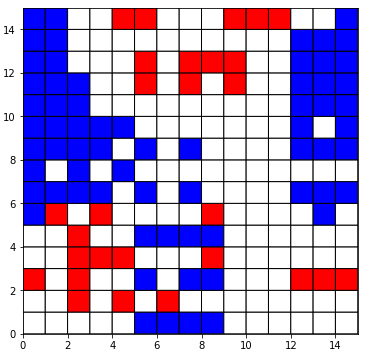
We can visualize the result of one step forward for arr:
1
2
3
4
5
6
7
arr = forward(arr, rules)
plt.figure(figsize=(6,6))
plt.pcolor(arr[::-1],
            cmap=cmap ,
            edgecolors=’k’,
            linewidths=1)
plt.show()

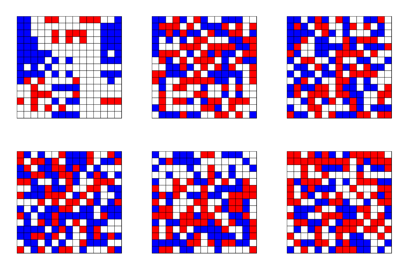
We can also generate and save a gif representing the evolution of the grid arr over many steps:
1
2
3
4
5
6
7
8
9
10
11
12
13
14
15
16
17
18
19
20
21
22
23
24
25
26
27
28
29
30
31
32
33
34
35
36
37
38
39
40
41
42
43
44
45
46
47
48
n_steps = 30
path = './gol.gif'
fps = 5


def generate_gif(n_steps, arr, rules,
                 path, cmap, figsize=(6, 6), fps=5):
  """
  Generate and save a gif to `path` corresponding
  to `n_steps`successive steps of evolution of
  `arr` according to `rules`
  :param n_step: int, number of steps to make the
    grid `arr` evolve
  :param arr: numpy array of the initial grid
  :param rules: dic, value => (surrounding, transitions)
  :param path: path where to save the resulting gif
  :param cmap: matplotlib cmap object. Must contain
    as many colors as possible values in `arr`
  :param figsize: size of each figure in the gif
  :param fps: frames per second for the resulting gif
  """
  images = []
  for i in range(n_steps):
  if i > 0:
    arr = forward(arr, rules)
  fig, ax = plt.subplots(figsize=(6, 6))
  ax.pcolor(arr[::-1],
            cmap=cmap,
            edgecolors='k',
            linewidths=1)
  ax.set_xticks([])
  ax.set_yticks([])
  # Used to return the plot as an image rray
  fig.canvas.draw() # draw the canvas, cache the renderer
  # Prevent each individual gif image to be displayed
  plt.close(fig)
  image = np.frombuffer(fig.canvas.tostring_rgb(),
                        dtype='uint8')
  image = image.reshape(fig.canvas.get_width_height()\
                        [::-1] + (3,))
  images.append(image)
  imageio.mimsave(path, images, fps=fps)
  print(f'INFO: gif saved to {path}')


generate_gif(n_steps, arr, rules, path, cmap,
             figsize=(6, 6),
             fps=5)

Multi-dimensional and multi-valued
Nothing prevents us to define the a game of life for say a 4-dimensional hypercube of dimension 15x20x30x10 with 5 possible values:
1
2
3
4
5
6
7
8
9
10
11
12
13
14
15
16
17
18
19
20
21
22
23
24
25
26
27
28
29
30
31
32
33
34
35
36
37
38
39
40
41
42
43
44
45
46
47
48
49
50
51
52
53
54
55
56
57
58
59
60
61
62
63
64
65
66
67
68
69
70
71
72
cmap = colors.ListedColormap(['blue', 'white', 'red',
                              'green', 'yellow', 'black'])
K, N, M, P = 15, 20, 30, 10

surrounding_0 = [(1, 0, 2, 1),
                 (-1, 0, 1, 3),
                 (0, 1, 0, 3),
                 (0, -1, 3, 1)]
surrounding_1 = [(1, 1, -2, 1),
                 (-1, -1, 1, 1),
                 (-1, 1, 1, 0),
                 (1, 3, -1, 4)]
surrounding_2 = [(1, 1, 2, 2),
                 (-1, -1, -1, 1),
                 (-1, 1, -1, 1),
                 (1, -1, 1, 1)]
surrounding_3 = [(1, 0, 0, 1),
                 (-1, 0, 1, 0),
                 (0, 1, 1, 0),
                 (0, -1, 1, -1)]
surrounding_4 = [(1, 1, 2, 1),
                 (-1, -1, 1, 2),
                 (-1, 1, 1, 1),
                 (1, 1, 2, -1)]
surrounding_5 = [(2, 1, 1, 0),
                 (-1, 2, -1, 1),
                 (-1, 1, 1, -1),
                 (1, 1, -1, -1)]

transitions_0 = [((0, 1), 1),
                 ((2, 3), 1),
                 ((4, 6), 3),
                 ((7, 9), 4),
                 ((10, np.inf), 0)]
transitions_1 = [((0, 2), 0),
                 ((3, 3), 1),
                 ((4, 10), 2),
                 ((11, np.inf), 1)]
transitions_2 = [((0, 2), 2),
                 ((3, 4), 1),
                 ((5, 6), 3),
                 ((7, 7), 1),
                 ((8, 8), 4),
                 ((9, np.inf), 5)]
transitions_3 = [((0, 1), 1),
                 ((2, 3), 1),
                 ((3, 6), 4),
                 ((7, 9), 5),
                 ((10, np.inf), 4)]
transitions_4 = [((0, 2), 0),
                 ((3, 3), 1),
                 ((4, 6), 4),
                 ((7, np.inf), 5)]
transitions_5 = [((0, 2), 2),
                 ((3, 4), 1),
                 ((5, 6), 2),
                 ((7, 7), 5),
                 ((8, np.inf), 2)]

rules = {
    0: (surrounding_0, transitions_0),
    1: (surrounding_1, transitions_1),
    2: (surrounding_2, transitions_2),
    3: (surrounding_3, transitions_3),
    4: (surrounding_4, transitions_4),
    5: (surrounding_5, transitions_5)
}

arr = np.random.randint(6,
                    size=K * N * M * P,
                    dtype=np.int8) \
                .reshape(K, N, M, P)
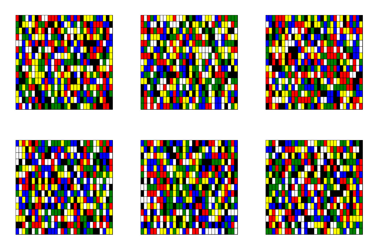
We can represent only a 2-dimensional slice of arr, so let’s draw for example the slice corresponding the the position 3 in the second dimension and position 4 in the fourth dimension, the same way than before, and we get:

As you can see, there are no much limitations to your imagination with this implementation.
Thank you for reading and have fun!