Hasenspiel - Escape the White Rabbit

Hasenspiel (German for “Rabbit Game”) is relatively simple game played on the chess board with 5 pawns. The goal is for the white pawn a.k.a. the rabbit to escape the opponent pawns. It’s a funny and not so trivial game. In this article, we will see how to completely solve it with an efficient implementation in C.

Game Rules

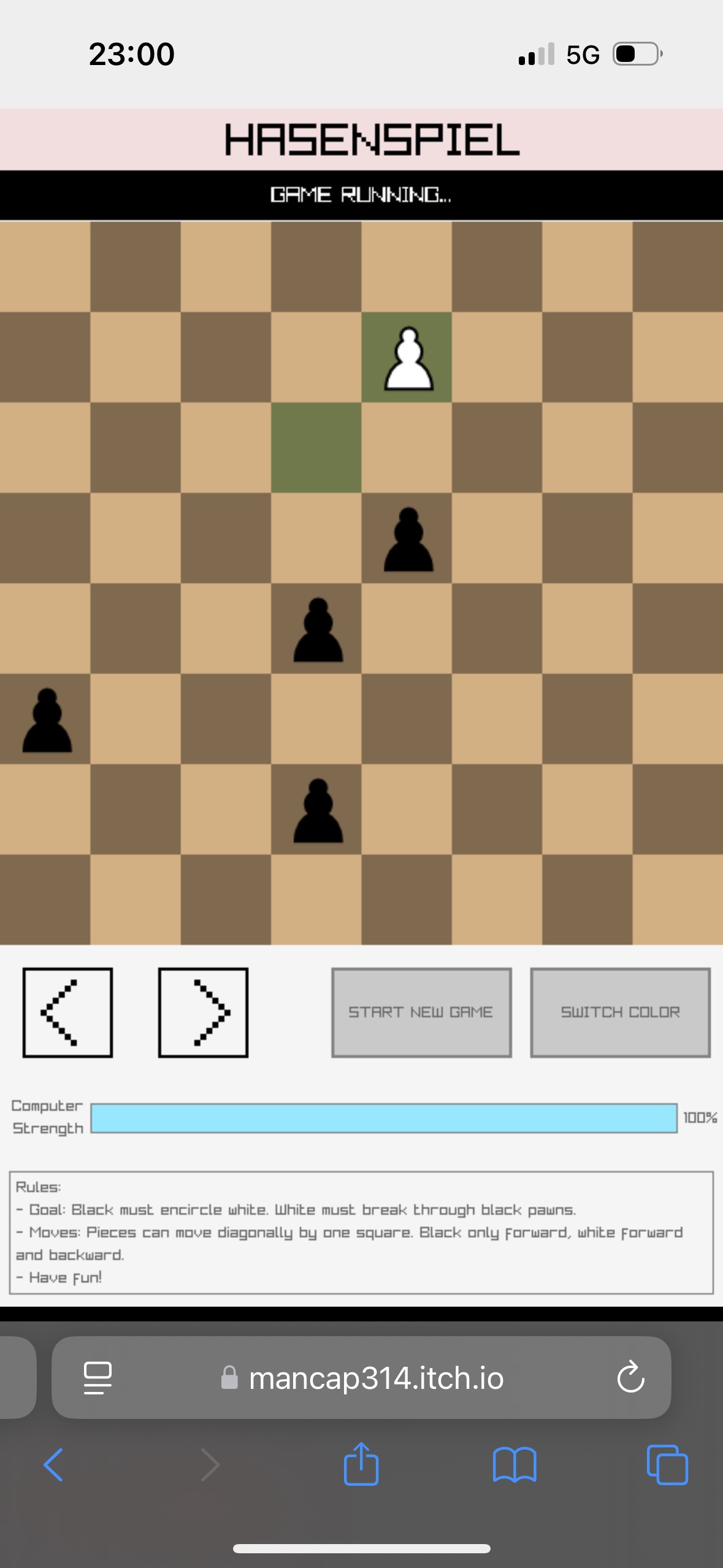
• Initial state: black has four pawns on the four black squares of the first raw. White has one pawn in a middle black square of the last opposite raw.
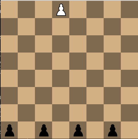
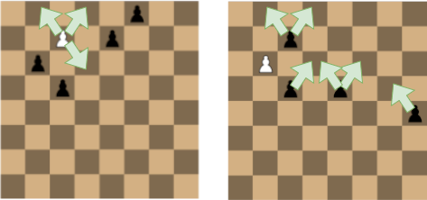
• Moves: white can move one square diagonally in every direction, besides it’s block by a board edge, or by a black pawn. Black can move one square diagonally, but only forward.

• The pawns can not jump over another pawn, and no pawn can be taken away from the board
• White starts, then black and white alternate turns. Black can move only one pawn at each turn.
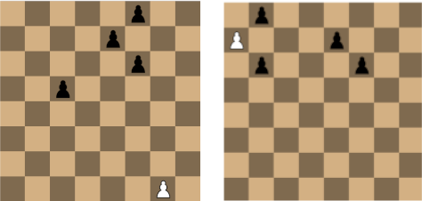
• Goal: White wins if it can reach the first raw: the rabbit has escaped. Black wins if it can completely block the white pawn.

Pretty easy so far.

Considerations on the Hasenspiel

The origin of this game is quite obscure. It was introduced to me by an acquaintance from Eastern Germany, thus it comes probably from there. I couldn’t find any resembling game searching on Google. If you are aware of one, please tell me.

This game is a good example of a Markov Decision Process (MDP) with two players and perfect information: all a player needs to know to decide a move lays open on the board. It has the Markov property, means the current state (board configuration + player on turn) is the only information required to estimate what could follow, no matter how this state was reached. Only the present state is relevant to make decisions, not the paste states. This has its importance in solving this game, as we will see later.

Other fact worth noticing: At the end of the game, there is one winner, and only one. No draw or whatever. This is also important in assessing if a player can force victory from a given position.

Last but not least: there is no exogenous randomness (e.g. dice roll) contributing to the game. Any state is the result of the decisions of the players only.

Questions

After playing a certain number of games, it seems however intuitive that black can force victory if it makes no mistake, but that it can easily make a mistake leading white to escape and win. Can we prove it?

The second question that arises is, can we define an optimal policy, means an optimal way to play at any given state for both black and white?

The third question is, how many possible states, means board configurations, are possible in this game? How many possible games are there?

Methodology

To answer those questions, we need to simulate all possible hasenspiel games. However, the number of possible games is too massive for a direct “bruteforce” approach. Thus the strategy is to follow a depth-first search (DFS) approach. White plays its forst possible move, then black its first possible move, etc. until the game reaches a final step where one of both players wins, from there we go up one step, explore the second last possible move, etc, until we have explored all possible nodes of the game. For each state, we store following information:

• If the player on turn at this state can force victory from there
• How many possible games there are from this state downward
• Among all those possible games, the percentage of them where black win

Nodes update

Nodes represent states. The children of a node are the states that can be reached from this state through the possible actions (moves) of the player at turn at this state. The nodes are updates recursively following the depth-first search, starting from the final nodes, where a player wins, backward to its parent node.

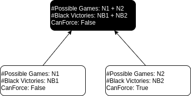
A final node has a number \(N=1\) of possible games, with a proportion \(p=1\) of winning games for the player that won at this node, and \(F=true\) for this winning player, means the player who wins there can force the victory there (obviously).

Then for a parent node:

• The number of its possible games is the sum of the possible games of its children node
• The number of winning games for black is the sum of the number of winning game for black of its children nodes.
• The player on turn at the parent node can force victory i.i.f. all the children nodes can’t force the victory, means its opponent has no possible move allowing him to force victory

If a node has already been evaluated during the search and is reached through another path: no need to go down this node again, you can re-use its already computed values. This is due to the Markov property mentioned above, and saves a massive amount of computation.

This way you go down to all the final nodes, up to the top node representing the start position, through all the intermediate nodes.

Answers

• Black can force victory from the start of the game, whatever white plays
• There are 1101.23 quintilions (quintillion: \(10^{27}\), or billions of billions of billions) possible games
• of which 54.59% where black wins
• There are 776,283 possibles states
• of which 39.45% where black can force victory, and 15.18% where white can force victory

And this was computed in… 0.148 seconds, on a single Intel(R) Core(TM) i5-10300H CPU @ 2.50GHz. Blazingly fast. See the next section.

Implementation

This program is implemented in C (code available here) and makes quite intensive use of bitwise operations and macro-functions. A quite common opinion is that macros are evil, or even programming masochism, but personally I like them. More on it on a next blog post maybe.

State representation

In every state of the game, all the pawns can only be on black squares, since they start on black square and can move only diagonally (easy inductive reasoning). There are 32 black squares on a standard chess board, numbered from 0 to 31, from left to right upward. Thus the position of a single pawn can be encoded in five bits (\(2^5=32\)), and the position of the five pawns on the board in 25 bits. Then, one more bit is required to encode the player at turn at this position. Thus 26 bits in total. This fits in a 32 bits unsigned integer type, a.k.a. uint32_t.

The position encoding is ordered as follows:

• First bit for the player at turn
• The five next bits for the position of the white pawn
• The next 20 bits for the position of the four black pawns, in descending order.

The descending order for encoding the position of the black pawns has two major advantages:

1. Position disambiguation: pawn 1 at position 4 and pawn 2 at position 8 for example is exactly the same as pawn 1 at position 8 with pawn 2 at 4. Thus by enforcing order, you prevent that various encodings encode the same position
2. The numerical value of the variable encoding the state is minimized, having the lowest value on the highest bits.

If white is at turn, it has max. 4 possible moves available (one move diagonally in every direction). Black has max. 8 possible moves. Thus all possible moves in any given state can be one-hot encoded in a single uint8_t variable.

Their are several pitfalls to be aware of, such as moves restricted for pawns on an edge, or move translation depending on the parity of the raw, e.g. move forward right means adding +4 to the position on even rows and +5 on odd rows. Also, when white wins, the game is not computed until it reaches the first row, but only until it passes by the last black pawn, where it is obvious that white is unstoppable from there. And many other tricks, leading to the performance mentioned above.

In order to store the immediate state, it suffices to note that the highest possible numerical value for a position encoding is \(60,614,406\). After subtracting the lowest possible numerical value of a position encoding, you get the size of the array where the nodes are stored during the depth-first search. As mentioned above, there are roughly 776k possible states, means nodes,so that this array stays quite sparse and there are probably ways to map the states in a narrower range of values.

Playing

When playing based on the states computed above, the agent evaluates the possible moves based and their resulting states, and their outlook for the opponent, in following priority:

• if a move results in a state where the opponent can force victory, it’s ranked lower than a move resulting in a state where the opponent can’t force victory.
• if two moves have the same effect on the opponent’s capacity to force victory, a move leading to a state where the opponent has a higher percentage of victory from all games starting from the resulting state, is ranked lower.

Thus the value of a move in a given position is evaluated based on its afterstate.

What we call here optimal policy, is when an agent (player) performs the resulting highest ranking action.

Conclusion

The Hasenspiel is a small game with interesting properties. It is way less complex than chess or go, but also way for complex than tic-tac-toe. Now that it’s completely solved, it allows to test various reinforcement learning approaches like Monte-Carlo, TD learning etc. in a setting where the ground-truth is known.

Its implementation shows also how to make aggressive use of macros and bitwise operations in a defensive programming style, for maximal performance and safety. The game is also easy to extend, for example changing the size of the board, or the number of black pawn. For this it’s enough to change the corresponding macro variables, and possible also switching from uint32_t to uint64_t for representing the states.

In the future I will maybe implement this game using Raylib, to have fun playing against the computer. Keep in touch.

Bonus: First 10 moves when bots agents play optimally

After a bit of experience in this game, it seems intuitively that the best strategy for black is to “keep the line”, means maintaining the black pawns on the same horizontal line as much as possible and moving this line forward. This way, the white rabbit has a hard time trying to escape. In the meanwhile, white moves to the middle and then tries to find a hole after coming in contact with black.

But surprizingly, when both players play optimally, white moves forward to the side, and black tries to catch him with only two pawns. See a picture of the first 10 moves when both players play optimally:

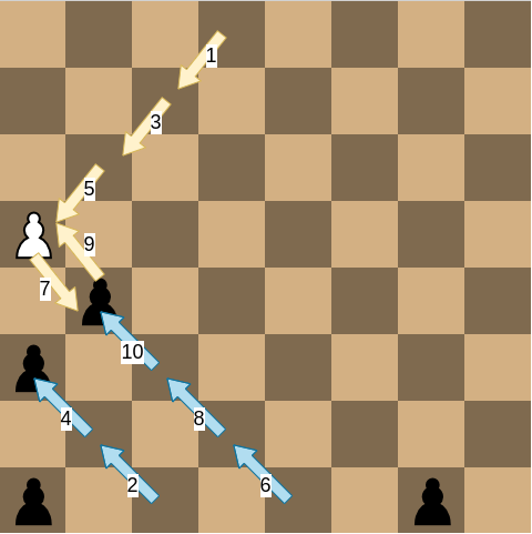
This is another example where the optimal strategy doesn’t match with the human intuition.

---

---